Welcome to the documentation for PHN!
This page provides a summary of the python functions used in in “Persistent Homology of Complex Networks for Dynamic State Detection” for generating and analyzing complex networks as the Persistent Homology of Networks (PHN). Additionally, a basic example is provided showing the functionality of the method for a simple time series. Below, a simple overview of the method is provided.
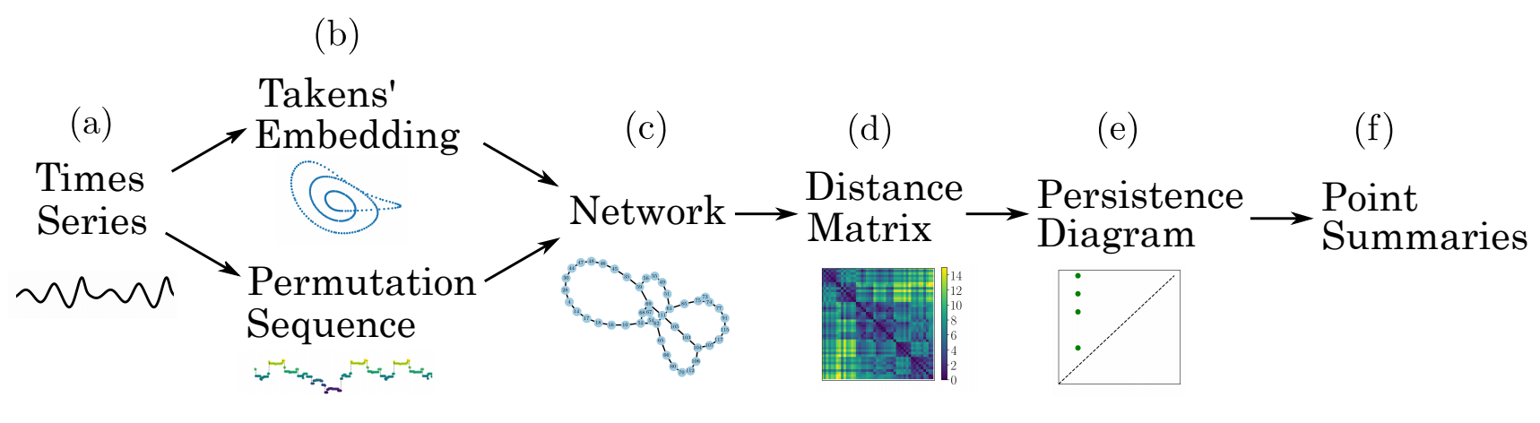
Outline of method: a time series (a) is embedded (b) using state space reconstruction from Takens’ embedding or segmenting the vectors into a set of permutations. From these two representations, an undirected, unweighted network (c) is formed by either applying a kth nearest neighbors algorithm or by setting each permutation state as a node. The distance matrix (d) is calculated using the shortest path between all nodes. The persistence diagram (e) is generated by applying persistent homology to the distance matrix. Finally, one of several point summaries (f) are used to extract information from the persistence diagram.
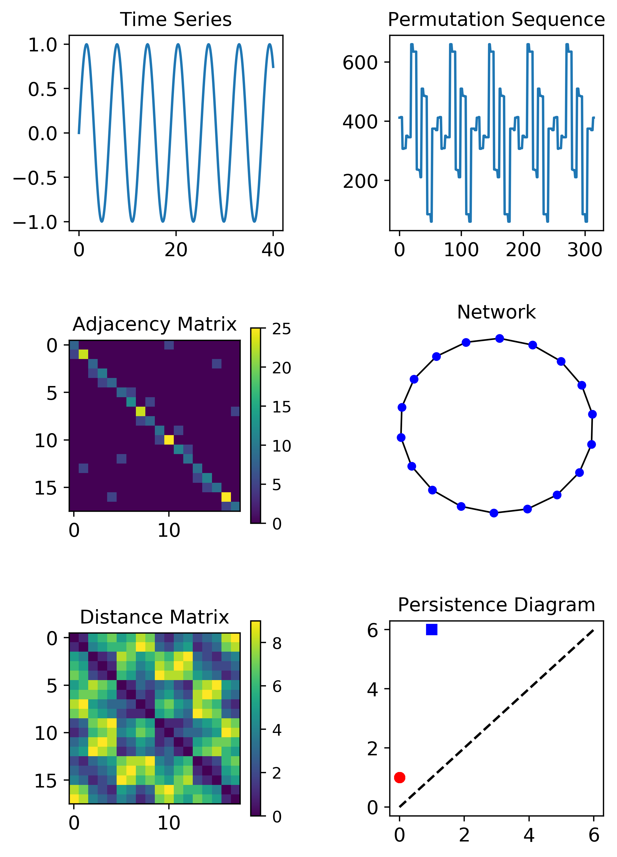
The following is an example implementing the method for an ordinal partition network for a simple time series:
from network_persistent_homology import PHN
import numpy as np
import matplotlib.pyplot as plt
import matplotlib.gridspec as gridspec
import networkx as nx
from scipy import sparse
from ripser import ripser

t = np.linspace(0,40,400)
ts = np.sin(t)

#example process for ordinal partition network
print('ORDINAL PARTITIONS METHOD')
tau = PHN.delay_op(ts)
n = 6
Sample = tau*100
ts = (ts)[0:Sample]
t = (t)[0:Sample]
#delay from embedding lag causing equiprobable permutations

#dimension from motif dimension with the highest permutation entropy per symbol
#However, n = 6 usually provides the best results.
print('delay:     ', tau)
print('dimension: ', n)

PS = PHN.Permutation_Sequence(ts,n,tau)
#Gets a sequence of permutations from time series

A = PHN.AdjacenyMatrix_OP(PS, n)
#gets adjacency matrix from permutation sequence transtitions

D = PHN.DistanceMatrix_OP(A, weighted = False, shortest_path = True)
#gets distance matrix from adjacency matrix with weighting as option and shortest path as option.

G, pos = PHN.MakeNetwork(A)
#makes graph from adjacency (unweighted, non-directional) matrix

D_sparse = sparse.coo_matrix(D).tocsr()
result = ripser(D_sparse, distance_matrix=True, maxdim=1)
diagram = result['dgms']


TextSize = 12
MS = 4
plt.figure(1)
plt.figure(figsize=(6,9))
gs = gridspec.GridSpec(3, 2)

ax = plt.subplot(gs[0, 0]) #plot time series
plt.title('Time Series', size = TextSize)
plt.plot(t, ts)
plt.xticks(size = TextSize)
plt.yticks(size = TextSize)

ax = plt.subplot(gs[0, 1]) #plot time series
plt.title('Permutation Sequence', size = TextSize)
plt.plot(PS)
plt.xticks(size = TextSize)
plt.yticks(size = TextSize)

ax = plt.subplot(gs[1, 0]) #plot time series
plt.title('Adjacency Matrix', size = TextSize)
plt.imshow(A)
plt.colorbar()
plt.xticks(size = TextSize)
plt.yticks(size = TextSize)

ax = plt.subplot(gs[2, 0]) #plot time series
plt.title('Distance Matrix', size = TextSize)
plt.imshow(D)
plt.colorbar()
plt.xticks(size = TextSize)
plt.yticks(size = TextSize)


ax = plt.subplot(gs[1, 1]) #plot time series
plt.title('Network', size = TextSize)
nx.draw(G, pos, with_labels=False, font_weight='bold', node_color='blue',
            width=1, font_size = 10, node_size = 20)

ax = plt.subplot(gs[2, 1]) #plot time series
plt.title('Persistence Diagram', size = TextSize)
plt.xticks(size = TextSize)
plt.yticks(size = TextSize)
plt.plot(diagram[0].T[0], diagram[0].T[1], 'ro')
plt.plot(diagram[1].T[0], diagram[1].T[1], 'bs')
plt.plot([0, max(diagram[1].T[1])], [0, max(diagram[1].T[1])], 'k--')


plt.subplots_adjust(hspace= 0.5)
plt.subplots_adjust(wspace= 0.5)
plt.show()
Where the output for this example is:
delay = 17
dimension = 6
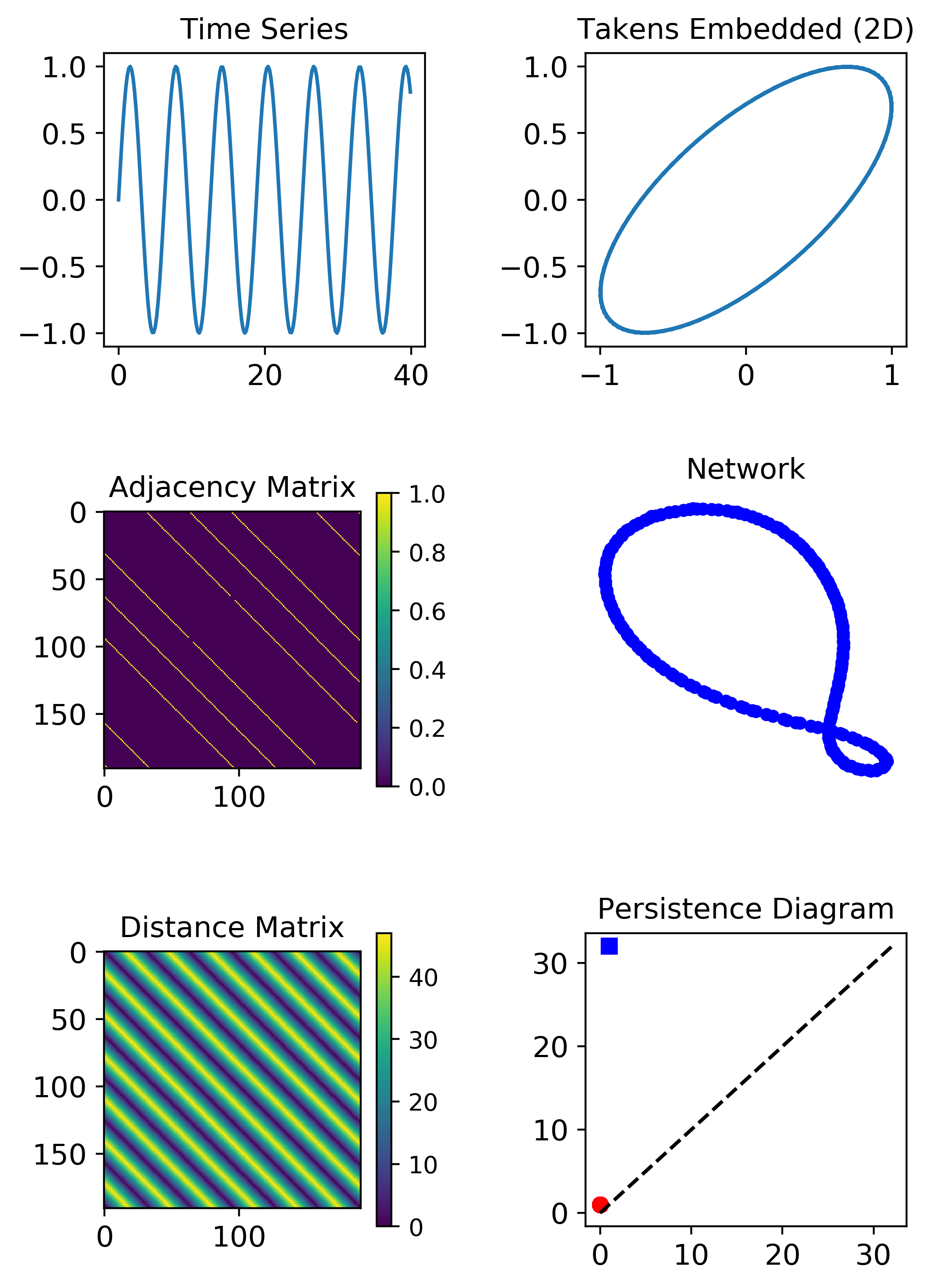
The following is an example implementing the method for a k-NN network for a simple time series:
from network_persistent_homology import PHN
import numpy as np
import matplotlib.pyplot as plt
import matplotlib.gridspec as gridspec
import networkx as nx
from scipy import sparse
from ripser import ripser

#example process for k nearest neighbors network from Takens' embedding

tau = PHN.MI_delay(ts)
#Mutual information isn't producing an accurate delay. Need to fix.
DownSample = tau/4 #downsampling to allow for longer time series
tau = int(tau/DownSample)
print('delay:     ', tau)
n = PHN.FNN_dim(tau,ts)+1
#embedding dimension from FNN +1 to make sure its high enough dimension
print('dimension: ', n)

sample = 300
t = t[::int(DownSample)][:sample]
ts = ts[::int(DownSample)][:sample]


emb_ts = PHN.Takens_Embedding(ts, n, tau)
#takens embedding of time series in n dimenional space with delay tau

distances, indices = PHN.k_NN(emb_ts, k= 4)
#gets distances between embedded vectors and the indices of the nearest neighbors for every vector

A = PHN.Adjacency_KNN(indices)
#get adjacency matrix (weighted, directional)

G, pos = PHN.MakeNetwork(A)
#get network graph based on adjacency matrix (unweighted, non-directional)

D = PHN.DistMatrix_KNN(A, distances, weighted = False, shortest_path = True)
#get distance matrix. Specify if weighting is desired or shortest path

D_sparse = sparse.coo_matrix(D).tocsr()
result = ripser(D_sparse, distance_matrix=True, maxdim=1)
diagram = result['dgms']


TextSize = 12
MS = 4
plt.figure(2)
plt.figure(figsize=(6,6))
gs = gridspec.GridSpec(3, 2)


ax = plt.subplot(gs[0, 0]) #plot time series
plt.title('Time Series', size = TextSize)
plt.plot(t,ts)
plt.xticks(size = TextSize)
plt.yticks(size = TextSize)

ax = plt.subplot(gs[0, 1]) #plot time series
plt.title('Takens Embedded (2D)', size = TextSize)
plt.plot(emb_ts.T[0],emb_ts.T[1])
plt.xticks(size = TextSize)
plt.yticks(size = TextSize)

ax = plt.subplot(gs[1, 0]) #plot time series
plt.title('Adjacency Matrix', size = TextSize)
plt.imshow(A)
plt.colorbar()
plt.xticks(size = TextSize)
plt.yticks(size = TextSize)

ax = plt.subplot(gs[2, 0]) #plot time series
plt.title('Distance Matrix', size = TextSize)
plt.imshow(D)
plt.colorbar()
plt.xticks(size = TextSize)
plt.yticks(size = TextSize)


ax = plt.subplot(gs[1, 1]) #plot time series
plt.title('Network', size = TextSize)
nx.draw(G, pos, with_labels=False, font_weight='bold', node_color='blue',
        width=1, font_size = 10, node_size = 20)


ax = plt.subplot(gs[2, 1]) #plot time series
plt.title('Persistence Diagram', size = TextSize)
plt.xticks(size = TextSize)
plt.yticks(size = TextSize)
plt.plot(diagram[0].T[0], diagram[0].T[1], 'ro')
plt.plot(diagram[1].T[0], diagram[1].T[1], 'bs')
if len(diagram[1].T[1]) > 0:
    plt.plot([0, max(diagram[1].T[1])], [0, max(diagram[1].T[1])], 'k--')


plt.subplots_adjust(hspace= 0.5)
plt.subplots_adjust(wspace= 0.5)
plt.show()
Where the output for this example is:
delay = 4
dimension = 3